<?xml version="1.0" encoding="utf-8"?><feed xmlns="http://www.w3.org/2005/Atom" ><generator uri="https://jekyllrb.com/" version="3.10.0">Jekyll</generator><link href="https://maksimrudnev.github.io/feed.xml" rel="self" type="application/atom+xml" /><link href="https://maksimrudnev.github.io/" rel="alternate" type="text/html" /><updated>2026-09-15T00:01:59+00:00</updated><id>https://maksimrudnev.github.io/feed.xml</id><title type="html">Elements of cross-cultural research</title><subtitle>by Maksim Rudnev</subtitle><entry><title type="html">Science versus Impact</title><link href="https://maksimrudnev.github.io/2026/08/04/science-versus-impact/" rel="alternate" type="text/html" title="Science versus Impact" /><published>2026-08-04T19:57:22+00:00</published><updated>2026-08-04T19:57:22+00:00</updated><id>https://maksimrudnev.github.io/2026/08/04/science-versus-impact</id><content type="html" xml:base="https://maksimrudnev.github.io/2026/08/04/science-versus-impact/"><![CDATA[<p>Every time I encounter a need to provide an impact statement or when I read for-impact studies, I get an ick because ‘impact’ and ‘science’ are barely related and often contradict each other. You can make a lot of impact without science. You can do science without any impact. Moreover, if you are doing science <em>for</em> impact, you are not doing science at all. Focus on the impact changes the subject from understanding to manipulation and, most importantly, compromises the method, which is a core of science.</p>

<!--more-->

<p>Researchers, of course, are rarely driven by pure curiosity, many pursue research for vanity, some do it to advance their careers or to achieve a certain impact. But these are confounders of science that should be controlled and balanced, not praised! These are essentially conflicts of interests, where pure curiosity and drive for understanding are being compromised. Can a conflict of interests pay for research and stimulate it? Yes, absolutely. Tobacco and oil businesses are eager to sponsor scientists. Is it a problem and does it question the results of this research? Unquestionably.</p>

<p>Likewise, when an academic runs an experiment to advance their career, they are committing to a wrong goal which inevitably leads to worse science. The examples are numerous, from the replication crisis to outright fraud to conscious bias. Open science framework is doing a great job at policing consequences of the wrong motivations, but it does not address the root cause of it – a system of wrong incentives.</p>

<p>The only motive making science possible is <a href="https://bsky.app/profile/maksimrudnev.com/post/3m5k3batfh22q">pure curiosity</a>, everything else should count as a potential conflict with pure curiosity. The other motivations, however virtuous and justified, lead to bias in science. When you write a paper to get a job, it’s a trap: you have better reasons to p-hack and fake the results rather than reporting real research outcomes. Doing science does not even require writing papers, it can be communicated through many other media, or even not communicated at all!</p>

<p>I think it is wildly misunderstood by university administrators, by funders, by general public, and even by many academics themselves (partly because universities and funders produce this kind of academics). Science isn’t just another industry and it cannot survive under the same system of incentives.</p>

<p>What is scientific about trying to find a drug that cures cancer? Colloquially there should be some ‘science behind’ it. Indeed, the pursuit of the drug puts the science <em>behind</em>, by putting the impact first. If some treatment suddenly works but we don’t know why, the aim of ‘finding a drug’ will be achieved but the science will not be advanced. <span style="font-size: 1rem;">Science begins when we start asking why this treatment worked.</span><span style="font-size: 1rem;"> ’Doing science’ is not virtuous, it’s innocent or even naïve.</span></p>

<p>While natural scientists can find refuge for their curiosity in formulas and abstract matters, in the social sciences, such <a href="/2017/06/30/conflict-of-interest-in-social-science/">conflicts of interests are much more problematic</a>, as research is centered on humans and tied to the applied Christian-humanistic values. If your main goal is fighting social inequality, your inequality research would be necessarily biased similar to a desperate student who <em>aims</em> to find statistical significance. Reflecting on consequences of your research is important (we don’t want another bomb) but failing to do so doesn’t make science less scientific  – whereas focus on consequences invalidates the scientific nature of activity.</p>

<p><span style="font-size: 1rem;">I understand that science needs a social interface, like a data center needs a user-friendly website. Science sometimes has to explain itself to the world. But the communication of the results is not a replacement for the substance: writing a paper is not a research outcome, it is no more equivalent to running an experiment than a logo on your shoes is equivalent to the shoes themselves. And the current ethos of academia puts communication – especially with increasingly general audiences – to the center, as it increases the audience size, and therefore citations, IF of journals, funding, and all sorts of social privileges that follow. Engagement of audiences depends on referring to issues they consider important, hence emphasis on societal impact, hence pivoting towards the ‘science-for-impact’. This is a dead end for science.</span></p>

<p>As maximalist and purist as some of the above may sound, I do believe these basic claims should be reiterated and reminded to everyone involved in and affecting science. I am not saying that science is somehow more valuable than ‘impact’, not at all, I am just saying that they are not even in the same family.</p>]]></content><author><name></name></author><category term="blog" /><category term="digressions" /><category term="philosophy" /><category term="purism" /><category term="science" /><summary type="html"><![CDATA[Every time I encounter a need to provide an impact statement or when I read for-impact studies, I get an ick because ‘impact’ and ‘science’ are barely related and often contradict each other. You can make a lot of impact without science. You can do science without any impact. Moreover, if you are doing science for impact, you are not doing science at all. Focus on the impact changes the subject from understanding to manipulation and, most importantly, compromises the method, which is a core of science.]]></summary></entry><entry><title type="html">Naming measurement instruments</title><link href="https://maksimrudnev.github.io/2025/04/24/naming-measurement-instruments/" rel="alternate" type="text/html" title="Naming measurement instruments" /><published>2025-04-24T20:45:03+00:00</published><updated>2025-04-24T20:45:03+00:00</updated><id>https://maksimrudnev.github.io/2025/04/24/naming-measurement-instruments</id><content type="html" xml:base="https://maksimrudnev.github.io/2025/04/24/naming-measurement-instruments/"><![CDATA[<blockquote>
  <div class="wp-caption aligncenter" style="width: 1546px">

<img class="wp-image-2234 size-full" src="/assets/images/uploads/2025/04/image-2.png" alt="" width="1536" height="1024" />

Although name Trikon reflects its owner's triangularity, Glopnik sounds way better.
</div>

  <p>When I first started studying psychology, I believed that the labels attached to psychological scales are trustworthy. Under this impression, I employed the scales based on what their names claimed to measure. Little did I know the labels and the content of scales are not (directly) related. Since then I lost my belief in scale names and simply skip to the items to get at least some idea of what it might be measuring.</p>
</blockquote>

<p><strong><em><span style="font-size: 1rem;">Jangle happens </span></em></strong></p>

<p><span style="font-size: 1rem;">Jingle-jangle fallacy has been raised so many times by this moment. To give a heads-up: jingle happens when you mistakenly buy an almond milk instead of a normal milk: both are named “milk” but have almost nothing to do with each other. Jangle happens when you order aubergine at a restaurant but they serve you eggplants—different names, same vegetable.</span></p>

<p><span style="font-size: 1rem;">Imagine you are trying to test criterion validity of your new Eggplant scale using an allegedly different Aubergine scale. How frustrating it is to realize that it’s the same thing and your attempt to prove validity generally fails because of that.</span></p>

<!--more-->

<p>New measurement instruments are normally developed in several steps beginning with a working definition of a construct. After that, normally, researchers generate stimuli/items, run trials and pilots, establish measurement properties and nomological networks, often<span class="Apple-converted-space">  </span>adjusting the instrument at every step: dropping items, modifying response points, changing its factor structure, so that the content of the initial pool of items is represented only partly and sometimes reduced dramatically to a single, not central, aspect of the construct of interest. Nevertheless, a theoretical construct assigned to the scale—as well as its name—stays the same as at the initial stage, even if the initially stated construct doesn’t have much to do with an actual scale content. Things get worse when the researcher feels creative and instead of initial ‘boring’ scale label proposes something click-bait-y (e.g., “dirty dozen”, “fascism”, “imposterism” scale). Some researchers suggest their teachers’ and heroes’ names to label their scale, or start using their own name to distinguish their scale from the others. Regardless how noble or narcissistic their motivation is, the result is the same—looking solely at the scale’s name, it’s impossible to say what it measures .<span class="Apple-converted-space"> </span></p>

<blockquote>
  <p>I guess it’s<span class="Apple-converted-space">  </span>not unique to scales, look at how people name their pets or even their very own children (Did you know there is a newborn in Kaliningrad, Russia whose first name is Putin? You might also heard of the former president of Ecuador who’s <a title="Lenín Moreno" href="https://en.wikipedia.org/wiki/Len%C3%ADn_Moreno">Lenín</a>).</p>
</blockquote>

<p>Quite often even decent informative scale names end up being acronyms which look more like Harry Potter spells (NEO-PI-R, HEXACO) or models of a deadly weapon<span class="Apple-converted-space"> </span>(MMPI-2-RF, WASI-II).</p>

<p><strong><em>What’s in a name?</em></strong></p>

<p>But it doesn’t have to be this way. Names could and should be able to help finding and using measurement instruments.</p>

<blockquote>
  <p>Names are given to identify what things are (i.e., provide a shortcut of their nature) and what they are not (i.e., distinguish from the others). For example, my name is Maksim which points to the fact that I am not, e.g.,  John, and its weird spelling (with -ks- instead of -x-) identifies my origin from a Slavic-speaking country.</p>
</blockquote>

<p>I suggest that scale naming should be based on the actual instrument’s content (as opposed to the initial idea, to what we <em>planned</em> to measure) and its distinguishing features (as opposed to marketing promise).</p>

<p>Imagine you started with an idea of a new flavour of right-wing-maga-conspiracy kind of a construct, but ended up with one factor and five items on prejudice against immigrants (e.g., “They’re eating the dogs”). It’s not a great idea to call it “MAGA scale” just because this title aligns with the initial idea and seems great for more attention and more citations. Such naming can only make the already pervasive jangle problem worse (remember eggplant?). So, following my own advice I would call it “anti-immigrant beliefs” and add something that makes it different from all the other (probably dozens of) similar scales, e.g., Anti-Immigrant Conspiracy Beliefs scale. On the other hand, I don’t want to duplicate the label, because it will cause a jingle issue (remember almond milk? uh, terrible). It’s likely that the naming issue will make me scan through the existing scales and I would conclude that such scale already exists. Yeah, wasted time, but at least we didn’t add to the jingle nor jangle.</p>

<p><strong><em>A rose by certain name</em></strong></p>

<p>The proliferation of poorly named measurement instruments isn’t just annoying—it actively hampers scientific progress. When researchers can’t efficiently locate appropriate scales or misunderstand what existing ones measure, we waste resources creating redundant tools and drawing faulty conclusions.</p>

<p>Scale names should function like good scientific labels: descriptive, distinctive, and honest about their content.  Ideally, it should be a convention, an APA standard if you will.</p>

<p>So the next time you develop a measurement instrument, resist the urge to name it after yourself, your mentor, or the latest cultural reference. Instead, do the unglamorous but scientifically sound work of naming it precisely for what it measures. Your future colleagues—desperately searching databases for appropriate scales—will silently thank you.</p>

<hr />

<p><em>1 Renaming <span style="text-decoration: underline;">existing</span> scales is very tempting but I am afraid it can create even bigger mess.</em></p>

<p><em>2 I believe psychological scales may stick for a while despite all the rapid technological change, so the naming issue will keep being important.</em></p>]]></content><author><name></name></author><category term="blog" /><category term="digressions" /><summary type="html"><![CDATA[Although name Trikon reflects its owner's triangularity, Glopnik sounds way better. When I first started studying psychology, I believed that the labels attached to psychological scales are trustworthy. Under this impression, I employed the scales based on what their names claimed to measure. Little did I know the labels and the content of scales are not (directly) related. Since then I lost my belief in scale names and simply skip to the items to get at least some idea of what it might be measuring. Jangle happens  Jingle-jangle fallacy has been raised so many times by this moment. To give a heads-up: jingle happens when you mistakenly buy an almond milk instead of a normal milk: both are named “milk” but have almost nothing to do with each other. Jangle happens when you order aubergine at a restaurant but they serve you eggplants—different names, same vegetable. Imagine you are trying to test criterion validity of your new Eggplant scale using an allegedly different Aubergine scale. How frustrating it is to realize that it’s the same thing and your attempt to prove validity generally fails because of that.]]></summary></entry><entry><title type="html">Presentation of our new paper on social status of older people around the world</title><link href="https://maksimrudnev.github.io/2023/02/18/presentation-of-our-new-paper-on-social-status-of-older-people-around-the-world/" rel="alternate" type="text/html" title="Presentation of our new paper on social status of older people around the world" /><published>2023-02-18T19:47:29+00:00</published><updated>2023-02-18T19:47:29+00:00</updated><id>https://maksimrudnev.github.io/2023/02/18/presentation-of-our-new-paper-on-social-status-of-older-people-around-the-world</id><content type="html" xml:base="https://maksimrudnev.github.io/2023/02/18/presentation-of-our-new-paper-on-social-status-of-older-people-around-the-world/"><![CDATA[<iframe width="560" height="315" src="https://www.youtube.com/embed/6rZsaxC5oJw" title="YouTube video player" frameborder="0" allow="accelerometer; autoplay; clipboard-write; encrypted-media; gyroscope; picture-in-picture; web-share" referrerpolicy="strict-origin-when-cross-origin" allowfullscreen=""></iframe>
<p>Rudnev, M., &amp; Vauclair, C. M. (2022).  <strong>Revisiting Cowgill’s Modernisation Theory: Perceived Social Status of Older Adults Across 58 Countries. </strong> <em>Ageing &amp; Society  </em> <a href="https://doi.org/10.1017/S0144686X22001192">https://doi.org/10.1017/S0144686X22001192</a> <a href="/assets/images/uploads/2022/10/2022-Status-of-older-adults-AS-accepted-version.pdf" rel="noopener">Full text</a></p>

<p><strong>Abstract</strong></p>

<p>Cowgill’s modernisation theory stipulates that older people’s social status is lower in societies with higher societal modernisation. The few existing studies reveal conflicting results showing either negative or positive associations. The current study follows up seminal cross-national research on the perceived social status of people in their seventies (PSS70) in a diverse set of countries. PSS70 was defined as the relative status of people in their seventies compared to people in their forties. Data were obtained by the World Values Survey (2010–2014) and included 78,904 respondents from 58 countries. Multilevel regressions showed that the level of modernisation had a strong and negative association with the PSS70 but mostly due to one component, namely the share of older people in society. The associations were more complex when considering cultural zones of which two stood out. Irrespective of level of modernisation, Muslim countries showed higher and post-communist countries showed lower levels of PSS70. In Muslim countries, modernisation had a near-zero association with PSS70, whereas it was strongly negatively associated with PSS70 in post-communist countries. This study generally supports Cowgill’s theory in a large and diverse cross-sectional sample of countries, yet it also illustrates its cultural boundary conditions.</p>]]></content><author><name></name></author><category term="blog" /><summary type="html"><![CDATA[Rudnev, M., &amp; Vauclair, C. M. (2022).  Revisiting Cowgill’s Modernisation Theory: Perceived Social Status of Older Adults Across 58 Countries.  Ageing &amp; Society   https://doi.org/10.1017/S0144686X22001192 Full text Abstract Cowgill’s modernisation theory stipulates that older people’s social status is lower in societies with higher societal modernisation. The few existing studies reveal conflicting results showing either negative or positive associations. The current study follows up seminal cross-national research on the perceived social status of people in their seventies (PSS70) in a diverse set of countries. PSS70 was defined as the relative status of people in their seventies compared to people in their forties. Data were obtained by the World Values Survey (2010–2014) and included 78,904 respondents from 58 countries. Multilevel regressions showed that the level of modernisation had a strong and negative association with the PSS70 but mostly due to one component, namely the share of older people in society. The associations were more complex when considering cultural zones of which two stood out. Irrespective of level of modernisation, Muslim countries showed higher and post-communist countries showed lower levels of PSS70. In Muslim countries, modernisation had a near-zero association with PSS70, whereas it was strongly negatively associated with PSS70 in post-communist countries. This study generally supports Cowgill’s theory in a large and diverse cross-sectional sample of countries, yet it also illustrates its cultural boundary conditions.]]></summary></entry><entry><title type="html">Alignment method for measurement invariance: Tutorial</title><link href="https://maksimrudnev.github.io/2019/05/01/alignment-tutorial/" rel="alternate" type="text/html" title="Alignment method for measurement invariance: Tutorial" /><published>2019-05-01T00:32:50+00:00</published><updated>2019-05-01T00:32:50+00:00</updated><id>https://maksimrudnev.github.io/2019/05/01/alignment-tutorial</id><content type="html" xml:base="https://maksimrudnev.github.io/2019/05/01/alignment-tutorial/"><![CDATA[<p>It’s been a while since measurement invariance alignment has been introduced in 2014, but not that many researchers applied it in practice. Among ~200 citations (as of May 2019) of the original alignment paper there were only a few substantive applications. It is a pity because you can always enjoy more optimistic results with alignment as compared to the conventional (frequentist, exact) measurement invariance techniques. I guess, it’s been happening due to statistical complexity and a lack of simple guidelines. In this post I summarized, in an approachable way, the steps that are necessary to apply alignment procedure. In addition, I provide <a href="/2019/05/01/alignment-tutorial/#extractAlignment">couple of  R functions</a> which automate preparation of Mplus code and extraction of useful information from the outputs.</p>

<p>Updates:</p>

<p>[August 23, 2023]: Please note this tutorial was based on Mplus version 7.3. Since then, Mplus developed many new features related to alignment and even introduced a <a href="https://www.statmodel.com/download/PML.pdf">new alignment-inspired class of models called penalized SEM</a>. [February 26, 2022]: Some minor errors were fixed. [November 13, 2020]: The post was updated to make it fully reproducible.</p>

<h2 id="contents">Contents</h2>

<p><a href="/2019/05/01/alignment-tutorial/#intro">Intro</a> <a href="/2019/05/01/alignment-tutorial/#step-1">Step 1. Find an acceptable configural invariance model</a> <a href="/2019/05/01/alignment-tutorial/#step-2">Step 2. Set up “FREE” alignment model in Mplus</a> <a href="/2019/05/01/alignment-tutorial/#step-3">Step 3. Set up “FIXED” alignment model</a> <a href="/2019/05/01/alignment-tutorial/#step-4">Step 4. Interpret the “Approximate measurement invariance” output</a> <a href="/2019/05/01/alignment-tutorial/#step-5">Step 5. Interpret “FACTOR MEAN COMPARISON” output</a> <a href="/2019/05/01/alignment-tutorial/#step-6">Step 6. Interpret “ALIGNMENT OUTPUT” output</a> <a href="/2019/05/01/alignment-tutorial/#step-7">Step 7. Checking the reliability of the results with simulation</a> <a href="/2019/05/01/alignment-tutorial/#files">Example Mplus files</a> <a href="/2019/05/01/alignment-tutorial/#additional">Additional options</a> (<a href="/2019/05/01/alignment-tutorial/#bayesian-estimation">Bayesian estimation</a>, <a href="#estimation-fine-tuning">estimation fine tuning,</a>  <a href="/2019/05/01/alignment-tutorial/#ranking-table">extra mean ranking table</a>, <a href="/2019/05/01/alignment-tutorial/#fit-function-contribution">fit function contribution,</a> <a href="/2019/05/01/alignment-tutorial/#categorical-indicators">categorical indicators</a>) <a href="/2019/05/01/alignment-tutorial/#software">Software</a>, including <a href="/2019/05/01/alignment-tutorial/#extractAlignment">automation in R</a> <a href="/2019/05/01/alignment-tutorial/#Resources">Resources</a></p>

<!--more-->

<h2 id="intro">Intro</h2>

<p>The typical start for applying alignment procedure is: ok, I tested my model for invariance with multiple group confirmatory factor analysis (MGCFA) and the equality of loadings and/or intercepts was rejected, so what’s next? Next goes one or some of the following:</p>

<p>If you believe that <span style="font-size: 1rem;">most parameters are invariant and few are non-invariant, try </span><strong>alignment</strong>, which will show you the possible set of groups in which invariance holds. It will also provide approximate latent means, even if there is no exact measurement invariance.</p>

<p>If you believe the model is likely to be invariant, but your data are noisy (i.e. many small meaningless intercorrelations of residuals, cross-loadings, etc.), consider applying  <strong>approximate invariance.</strong> It is based on Bayesian statistics and allows small differences in loadings/intercepts across groups. One sign to apply approximate approach is when you experience problems even with configural invariance model (but you are sure your model is properly specified).</p>

<p>If you believe that most parameters are invariant AND your data are noisy, there is an option of <strong>Bayesian alignment</strong>, which combines approximate invariance (or simply Bayesian estimation) with alignment approach. I describe it in <a href="#bayesian-estimation">section 8</a>.</p>

<p>In case your data contain very many groups (&gt;100), consider using <strong>multilevel CFA</strong> with random loadings and intercepts (<a href="https://doi.org/10.1177/0049124117701488">random effects model</a>).</p>

<p>At some point you might <strong>admit</strong> there is no invariance at least for some groups. So I would usually try to <strong>explain</strong> why there is no invariance. You may speculate about differences in meaning, make cognitive interviews to understand it, or explain non invariance by applying multilevel CFA with a group-level covariate as in <a href="https://doi.org/10.1177/0022022112438397">Davidov et al. 2012</a>.</p>

<p>Below, I focus on alignment method in Mplus software. Alignment estimates a configural invariance model and then modifies the factor loadings and intercepts to make them as similar  across groups as possible without deteriorating the model fit. Conceptually, the procedure is alike target factor rotation where the target is across-group similarity of loadings and intercepts.</p>

<h2 id="step-1">Step 1. Find an acceptable configural invariance model</h2>

<p>This is crucial as the alignment procedure is based on configural model and the models with aligned parameters  have the same fit (alignment doesn’t affect fit, similar to factor rotation). If the fit of configural model is not good enough, consider fitting the configural model using Bayesian approach and testing approximate Bayesian invariance (probably with further alignment). Dropping items and groups are the hardcore measures, apply them only if it is reasoned substantively.</p>

<p><strong>My example:</strong> I use the data from <a href="http://www.worldvaluessurvey.org/WVSDocumentationWV5.jsp">World Values Survey wave 5</a>  (<a href="/files/Align_prepare_data.R">the sample was shrunk</a> to 10 convenient countries for the speed of computation). The model is a single factor of sexual and reproductive morality. It has 4 indicators: justifiability of homosexuality, prostitution, abortion, and divorce. The residuals of abortion and divorce items are allowed to covary. The configural measurement invariance model <a href="/files/exact_manual.out">shows</a> an acceptable model fit ( CFI = 0.995, RMSEA = 0.072) however, constraining factor loadings across groups – that is, setting up a metric invariance model – ruins the fit (CFI = 0.969, RMSEA = 0.094). So  I have to reject the metric invariance hypothesis. However, a good fit of configural model gives some hope so I can reach for the alignment procedure.</p>

<p>Before going further, keep in mind that alignment cannot handle cross-loadings (as well as anything beside factor model <span style="color: #ff0000;">[update: this limitation is no longer present with Mplus versions starting from 8.8]</span>), but it is fine to have residual covariances. It can also deal with categorical (binary and ordinal) indicators.</p>

<h2 id="step-2">Step 2. Set up “FREE” alignment model in Mplus</h2>

<p>There are two kinds of alignment models, Free and Fixed, they differ in the set of constraints placed on the MGCFA model. It is advised to run, first, Free alignment, and then for go for the Fixed one.</p>

<p>In general, the Free model works better with a large non-invariance, so if this model doesn’t converge, skip to the next step.</p>

<p>Mplus code would look like this:</p>

<div class="language-plaintext highlighter-rouge"><div class="highlight"><pre class="highlight"><code>DATA: file = 'mplus_data.tab';
VARIABLE: 
  NAMES = country prostit homosex abortion divorce; 
  MISSING=.;
  classes = c(10);! Type a number of groups in your data in parentheses  
     knownclass = c(country =  36   ! Australia
                             76   ! Brazil
                             124  ! Canada
                             170  ! Colombia
                             380  ! Italy
                             554  ! New Zealand 
                             642  ! Romania
                             643  ! Russia
                             792  ! Turkey
                             840  ! United States
   );
! The classes are not actually latent, they are *known* and 
! it is just a grouping variable. So place the grouping variable  
! on the place of 'country' above and list the categories in 
! this variable (list all groups). Also, Mplus doesn't handle 
! string names of groups, so we have to deal with numeric codes

ANALYSIS:
  TYPE = mixture; ! Actually it is a multiple group model, 
                  ! but for technical reasons is specified as a mixture.   
  ESTIMATOR = ml; ! it can be mlr or mlf, or Bayes as well. See Section 8   
  ALIGNMENT = FREE; ! this line makes Mplus to actually run alignment.

MODEL:
    %OVERALL% ! it means the CFA model specified below is applicable in every group
     Moral BY prostit homosex abortion divorce;
     abortion WITH divorce;

OUTPUT: 
   align; ! This line requests the detailed info on alignment
</code></pre></div></div>

<h2 id="step-3">Step 3. Set up “FIXED” alignment model</h2>

<p>In the <a href="/files/free_manual.out">output</a> of the previous “free alignment” model you can find a message -</p>

<div class="language-plaintext highlighter-rouge"><div class="highlight"><pre class="highlight"><code>STANDARD ERROR COMPARISON INDICATES THAT THE FREE ALIGNMENT MODEL MAY BE POORLY IDENTIFIED.
     USING THE FIXED ALIGNMENT OPTION MAY RESOLVE THIS PROBLEM.
     TO AVOID MISSPECIFICATION USE THE GROUP WITH VALUE 792 AS THE BASELINE GROUP.
</code></pre></div></div>

<p>It is self-explaining: follow this recommendation and replace in the above Mplus input the <span class="fn">ANALYSIS</span> section line <span class="fn">ALIGNMENT = FREE;</span> with the line <span class="fn">ALIGNMENT = FIXED(792);</span> and put the number of group  in parentheses with the one recommended by Mplus (it is just the smallest estimated latent mean). Sometimes Mplus doesn’t suggest specific group, so you can just choose the one with the smallest latent mean(s). Run this new code.</p>

<h2 id="step-4">Step 4. Interpret the “Approximate measurement invariance” output</h2>

<p>In the <a href="/files/fixed_manual.out">output</a> you will find this specific section of the alignment results. Here’s an excerpt from the fixed alignment:</p>

<div class="language-plaintext highlighter-rouge"><div class="highlight"><pre class="highlight"><code>APPROXIMATE MEASUREMENT INVARIANCE (NONINVARIANCE) FOR GROUPS

Intercepts/Thresholds
   PROSTIT     36 76 124 170 380 554 (642) 643 792 840
   HOMOSEX     36 (76) (124) (170) 380 554 (642) (643) 792 840
   ABORTION    36 (76) 124 (170) 380 554 (642) (643) 792 840
   DIVORCE     36 (76) 124 170 380 554 642 (643) (792) 840

Loadings for MORAL1
   PROSTIT     (36) 76 (124) (170) (380) 554 642 643 792 (840)
   HOMOSEX     36 76 124 170 380 554 (642) 643 (792) 840
   ABORTION    (36) 76 (124) 170 380 554 642 643 (792) (840)
   DIVORCE     36 76 124 (170) 380 554 642 643 792 840
</code></pre></div></div>

<p>It can be hard to read, but it is meant to simplify the results: this is the table of the intercepts and loadings compared across groups. The groups in which this current parameter is NOT invariant even after alignment are in parentheses. In my example,  intercept of PROSTIT indicator is significantly different in group 642, while in the other groups they are approximately the same. Likewise, the loading of DIVORCE is non-invariant in group 170, while in the other groups this loading is invariant. The parameters are compared across groups using a convenient confidence level of 95%.</p>

<h2 id="step-5">Step 5. Interpret “FACTOR MEAN COMPARISON” output</h2>

<div class="language-plaintext highlighter-rouge"><div class="highlight"><pre class="highlight"><code>FACTOR MEAN COMPARISON AT THE 5% SIGNIFICANCE LEVEL IN DESCENDING ORDER

Results for Factor MORAL1

Latent    Group      Factor
 Ranking    Class    Value       Mean     Groups With Significantly Smaller Factor Mean
     1         1        36       2.432    554 124 840 76 380 643 170 642 792
     2         6       554       2.154    124 840 76 380 643 170 642 792
     3         3       124       1.773    840 76 380 643 170 642 792
     4        10       840       1.545    76 380 643 170 642 792
     5         2        76       0.855    643 170 642 792
     6         5       380       0.823    643 170 642 792
     7         8       643       0.522    170 642 792
     8         4       170       0.347    792
     9         7       642       0.303    792
    10         9       792       0.000
</code></pre></div></div>

<p>For each factor in the model, alignment would produce this comparison of the estimated means. The same information in a different form can be requested by <a href="#ranking-table">RANKING</a> option of the OUTPUT section.</p>

<p><strong>!! Be careful,</strong> these are the latent means that are estimated <em>ignoring</em> measurement non-invariance, it doesn’t mean they are reliable or fully invariant, they were estimated just for reference. These can be treated seriously <em>only</em> if the other tests support approximate measurement invariance.</p>

<p>First column is rank of the mean, second is internal number of group,  third one is your code of the group.</p>

<p>The last column of the table provides pairwise comparison of every group’s mean  with all the other groups’ means.  In the example, country 36 (Australia) has the highest values on the latent mean, and it significantly differs from all the other countries. You can find the same means in the upper parts of the output, in the MODEL RESULTS section.</p>

<h2 id="step-6">Step 6. Interpret “ALIGNMENT OUTPUT”</h2>

<p>This section will be produced if you add to the input code line <span class="fn">OUTPUT: ALIGN;</span>. It provides detailed information on the results of alignment for each parameter.  For each parameter, it shows three things: pairwise  comparison, summarized invariance information, and parameter values that were aligned across groups.</p>

<h3 id="step-6-1">6.1. Pairwise comparison</h3>

<p>First, it is a large table which begins like this:</p>

<div class="language-plaintext highlighter-rouge"><div class="highlight"><pre class="highlight"><code>ALIGNMENT OUTPUT

INVARIANCE ANALYSIS

Intercepts/Thresholds
 Intercept for PROSTIT
  Group     Group      Value      Value     Difference  SE       P-value
     76        36      1.613      1.606      0.006      0.056      0.912
     124       36      1.627      1.606      0.021      0.077      0.788
     124       76      1.627      1.613      0.015      0.043      0.735
     170       36      1.650      1.606      0.043      0.066      0.508
     170       76      1.650      1.613      0.037      0.029      0.204
     170       124     1.650      1.627      0.023      0.055      0.680
     380       36      1.638      1.606      0.032      0.074      0.669
     380       76      1.638      1.613      0.025      0.042      0.543
     380       124     1.638      1.627      0.011      0.059      0.853
     380       170     1.638      1.650     -0.012      0.051      0.819
     554       36      1.532      1.606     -0.074      0.104      0.476
     &lt;...&gt;
</code></pre></div></div>

<p>This table compares parameters and statistically tests their equality across each possible pairs of groups. First line in this example compares Intercept for PROSTIT in group 76 and in group 36,  the intercept in group 76 is 1.613 and the intercept in group 36 is 1.606, and we can see that the difference is 0.006 which is far from being significant. Yihaa, we found one invariant parameter across two groups. If only always it worked like this. This table can be really large, because there is every possible pair of groups, so for 10 groups there will be 45 lines <em>for each</em> parameter. This table provides a very detailed information, so I would ignore it at this stage and return to it only in case other things fail to help.</p>

<h3 id="step-6-2">6.2. Summarized invariance info</h3>

<div class="language-plaintext highlighter-rouge"><div class="highlight"><pre class="highlight"><code> Approximate Measurement Invariance Holds For Groups:
 36 76 124 170 380 554 643 792 840
</code></pre></div></div>

<p>Below the pairwise comparisons there is a list of groups in which this current parameter was found invariant after alignment. We already seen this information above, at <a href="#step-4">Step 4</a>. Sometimes, it is not very useful, especially if you have many groups and only few of them are non-invariant – imagine trying to identify group(s) which is absent from the list (answer here - group 642). So just ignore it and refer to the above <a href="#step-4">Step 4</a>.</p>

<div class="language-plaintext highlighter-rouge"><div class="highlight"><pre class="highlight"><code>Weighted Average Value Across Invariant Groups:       1.628
</code></pre></div></div>

<p>This is an aligned value that can be considered common for all the invariant groups, listed at a previous line. Note that this value is applicable <em>only</em> to the invariant groups!</p>

<div class="language-plaintext highlighter-rouge"><div class="highlight"><pre class="highlight"><code>R-square/Explained variance/Invariance index:       0.916
</code></pre></div></div>

<p>This R² indicates a degree of invariance of the given parameter. <a id="back-from-footnote" href="https://doi.org/10.1177/0049124117701488">Muthén</a> interpreted this index as the degree to which “<span style="font-size: 1rem;">the variation across groups in the configural model intercepts and loadings for this item is explained by variation in the factor mean and factor variance [respectively] across groups.” A little confusing can be the fact that this R² can be really small even if the corresponding parameter is highly invariant</span><a style="font-size: 1rem; color: #0f3647;" href="#footnote">*</a><span style="font-size: 1rem;">.</span><span style="font-size: 1rem;"> In my example, the factor loading of indicator PROSTIT was shown to be invariant across 9 out of 10 groups, and accrodingly R² is quite high 0.916.</span></p>

<h3 id="step-6-3">6.3. Aligned parameter values</h3>

<div class="language-plaintext highlighter-rouge"><div class="highlight"><pre class="highlight"><code>Invariant Group Values, Difference to Average and Significance
 Group        Value Difference         SE    P-value
     36       1.606     -0.022      0.054      0.687
     76       1.613     -0.016      0.012      0.184
     124      1.627     -0.001      0.039      0.976
     170      1.650      0.022      0.028      0.433
     380      1.638      0.010      0.041      0.813
     554      1.532     -0.096      0.067      0.152
     643      1.595     -0.034      0.011      0.003
     792      1.753      0.125      0.042      0.003
     840      1.600     -0.028      0.049      0.566
</code></pre></div></div>

<p>Here, the parameter estimates are listed, but only for those groups which were found to be invariant (e.g. line with group 642 isn’t here). This table is meant to demonstrate the invariance of the invariant parameter. That’s why the values of parameters in the non-invariant groups are not included in this table (but you can find them in the main output “MODEL RESULTS” where all the parameters are listed).</p>

<h3 id="step-6-4">6.4. Average Invariance index</h3>

<p>The tables 6.1-6.3 are repeated for each factor loading and each indicator intercept. In the very end of the Alignment Output you will find</p>

<div class="language-plaintext highlighter-rouge"><div class="highlight"><pre class="highlight"><code>Average Invariance index: 0.671
</code></pre></div></div>

<p>This is an average R² across all the parameters. It is a handy global score of both metric and scalar invariance. Here, 1 stands for perfect scalar invariance, 0 for (likely impossible) full non-invariance. In general, one may interpret this index as a degree of confidence to which the means can be meaningfully compared across the given set of groups.</p>

<h2 id="step-7">Step 7. Checking the reliability of the results with simulation</h2>

<p>The issue with alignment is that it is tied to a current dataset, so its external validity is questionable. For example,  if you have small samples within groups the standard errors of the loadings may be underestimated, so the alignment can find an invariance where it is not present. To check if this is the case, it is recommended to run a simulation study. It was made quite easy by Mplus.</p>

<h3 id="step-7-1">7.1. Set up a simulation study</h3>

<p>First, you need to re-run your last alignment model adding to the section <span class="fn">OUTPUT</span>, a command <span class="fn">SVALUES</span>, which will print the parameter estimates in the form of input commands for simulation study.  After running this updated code, navigate the output to the section “MODEL COMMAND WITH FINAL ESTIMATES USED AS STARTING VALUES” and copy the whole section (it is usually very large).</p>

<p>Next, you need to make several modifications to it: (a) remove intercepts part from the %OVERALL%  section, add starting values to loadings in this section, and replace C# with G# in the names of classes. Below the changes are in red.</p>

<div class="language-plaintext highlighter-rouge"><div class="highlight"><pre class="highlight"><code> %OVERALL%

moral BY prostit*1;  ! Added *1 for every loading
     moral BY homosex*1;
     moral BY abortion*1;
     moral BY divorce*1;

 [ c#1*0.16328 ];
[ c#2*0.23189 ];
[ c#3*0.59097 ];
[ c#4*0.93735 ];
[ c#5*-0.16690 ];
[ c#6*-0.29107 ];
[ c#7*0.36642 ];
[ c#8*0.51571 ];
[ c#9*0.12452 ];;

%CG#1% ! This change should be done for the rest of the code as well

moral1 BY prostit*1.26506;
     moral1 BY homosex*1.51873;
     moral1 BY abortion*1.37710;
     moral1 BY divorce*1.07074;

abortion WITH divorce*1.03434;

[ prostit*1.60633 ];
&lt;...&gt;
</code></pre></div></div>

<p>Okay, now we are ready to combine it with the simulation code.</p>

<p>Next, create a new input file</p>

<div class="language-plaintext highlighter-rouge"><div class="highlight"><pre class="highlight"><code>MONTECARLO:
NAMES = prostit homosex abortion divorce; ! Names of indicator variables (only)
ngroups = 10; ! Your number of groups
NOBSERVATIONS = 10(100); ! This is again a number of groups and sample size of each group in parentheses.
NREPS = 500; ! This is how many times the data generation and analysis should be repeated.

ANALYSIS:
TYPE = MIXTURE;
ESTIMATOR = ml;
alignment = fixed(9); ! a order number of the group in which the mean was fixed to 0 (it was 736=Turkey in the Step 3, and it's 9th group in the specification of knownclas
MODEL POPULATION:! This section includes a model to generate data

! Paste here the code that we created just before using svalues output
! - it looks like this:
       %OVERALL%
       moral BY prostit*1;
       moral BY homosex*1;
       moral BY abortion*1;
       moral BY divorce*1;

%g#1%

moral1 BY prostit*1.26506;
     moral1 BY homosex*1.51873;
       &lt;...&gt;

MODEL: ! This section includes a model to analyze

! AND again, paste here the same edited svalues code -  

%OVERALL%
       moral BY prostit*1;
       moral BY homosex*1;
       moral BY abortion*1;
       moral BY divorce*1;

%g#1%

moral1 BY prostit*1.26506;
     moral1 BY homosex*1.51873;
       &lt;...&gt;
</code></pre></div></div>

<p>And run it. It will take some time. Save the output, change the sample size in the parentheses of NOBSERVATIONS = 10(500); and run again. Then change the sample size again and run again. You will end up with three or more outputs based on different sample sizes. It will demonstrate if the model is able to reproduce the latent means with the data of different sample size.</p>

<h3 id="step-7-2">7.2. Interpret outputs of the simulation</h3>

<p>Locate in the <a href="/files/simulation100_manual.out">output file</a> the following tables:</p>

<div class="language-plaintext highlighter-rouge"><div class="highlight"><pre class="highlight"><code>CORRELATIONS AND MEAN SQUARE ERROR OF POPULATION AND ESTIMATE VALUES

CORRELATIONS                MEAN SQUARE ERROR
                    Average    Std. Dev.           Average    Std. Dev.
 MORAL1
    Mean             0.9716      0.0151             0.2854       0.101
    Variance         0.7738      0.1566             1.2841      14.002

CORRELATION AND MEAN SQUARE ERROR OF THE AVERAGE ESTIMATES

MORAL1 Mean                         0.999        0.045
         MORAL1 Variance                     0.457        0.724
</code></pre></div></div>

<p>These are two sets of measures of reliability of latent means estimated in the previous steps with alignment. First table results from two-stage computation:</p>

<ol>
  <li>it extracts latent means in across groups, which were estimated in a single simulation and correlates them to the true (population) means, and then</li>
  <li>these correlations are averaged across all the simulations (in my case 500).</li>
</ol>

<p>In the same way, the measure is found for the latent variances. Std. Dev. of correlations/variances here refers to standard deviation of correlations across simulation runs. It seems correct to interpret these scores as a measure of reliability of latent means estimated by alignment. These correlations are typically very high, so I would be worried when they are less than 0.95 (<a href="https://www.statmodel.com/download/PolAn.pdf">Asparouhov and Muthen, 2013</a> suggest that correlations should be not less than 0.98). In my example, there is something disturbing going with the estimated variances. However, when I run <a href="/files/simulation1500_manual.out">a simulation with 1500 cases</a> in each simulation (which is closer to my actual data) this correlation gets very close to 1 (0.998). It means that such a model wouldn’t work if I had  less respondents.</p>

<p>Additionally, mean square error is calculated, which is an absolute reverse measure of association.</p>

<p>Second table is a product of</p>

<ol>
  <li>averaging latent means across all the simulation runs (500 in my case), and</li>
  <li>correlating it with the true values.</li>
</ol>

<p>First column lists these correlations, the second column is (apparently) mean square error. These measures seem to indicate reliability of the simulation itself, and reliability of the measurement model in general.</p>

<p>Sometimes all these correlations are zeros. If this is the case scroll down to the errors section; it might be that the model was misspecified somehow or none of the models converged.</p>

<p>That’s it.</p>

<p>If the news are good and alignment helped to locate problematic parameters/groups, you may proceed with corresponding dropping groups/modifying model to achieve higher levels of invariance. If you are happy with what you get with alignment, next step might be predicting factor scores based on alignment and then using them as a reliable (though not perfect) substitute of the factor scores. It can be done in a standard Mplus way by adding <span style="font-size: 1rem;"><span class="fn">SAVE = FSCORES;</span> to the <span class="fn">SAVEDATA:</span> section.</span></p>

<h2 id="files">Example Mplus files</h2>

<p>Here is the list of the files used in the examples above</p>

<ul>
  <li><a href="/files/mplus_data.tab">mplus_data.tab</a></li>
  <li><a href="/files/free_manual.inp">free_manual.inp</a></li>
  <li><a href="/files/free_manual.out">free_manual.out</a></li>
  <li><a href="/files/fixed_manual.inp">fixed_manual.inp</a></li>
  <li><a href="/files/fixed_manual.out">fixed_manual.out</a></li>
  <li><a href="/files/simulation100_manual.inp">simulation100_manual.inp</a></li>
  <li><a href="/files/simulation100_manual.out">simulation100_manual.out</a></li>
  <li><a href="/files/simulation500_manual.inp">simulation500_manual.inp</a></li>
  <li><a href="/files/simulation100_manual.out">simulation500_manual.out</a></li>
  <li><a href="/files/simulation1500_manual.inp">simulation1500_manual.inp</a></li>
  <li><a href="/files/simulation1500_manual.out">simulation1500_manual.out</a></li>
</ul>

<h2 id="additional">Additional options</h2>

<h3 id="bayesian-estimation">Bayesian estimation</h3>

<p>This is pretty much uncharted territory because only a few publications explored this analysis. One may consider using Bayesian alignment if the data are noisy and even configural model does not show a great fit to the data. The next step in this case would be setting up a Bayesian approximate invariance model with small prior variances of parameters across groups, and next running the alignment to find better solution. Check <a href="https://www.frontiersin.org/articles/10.3389/fpsyg.2015.01963/full">this paper</a> with its supplementary materials for the full example. Another option is to simply substitute maximum likelihood with Bayesian estimation (it requires adding <span class="fn">ESTIMATOR: BAYES;</span> in the <span class="fn">ANALYSYS:</span> section). From my experience, the latter way produces less errors and overall problems compared to ML estimation.</p>

<h3 id="ranking-table">Ranking table</h3>

<p>You can request it by adding <span class="fn">SAVEDATA: RANKING IS ranking.dat;</span> in the input file of fixed or free alignment (not simulation). The rankings of groups are based on the freely estimated and aligned group factor means, the differences are determined by the significance of the factor mean differences. It is also listed in the standard output, but in a bit different form, as shown in <a href="#step-5">Step 5</a> ”Factor mean comparison”.</p>

<div class="language-plaintext highlighter-rouge"><div class="highlight"><pre class="highlight"><code>Ranking table for MORAL1

,36,554,124,840,76,380,643,170,642,792,
36,X,&gt;,&gt;,&gt;,&gt;,&gt;,&gt;,&gt;,&gt;,&gt;,
554,&lt;,X,&gt;,&gt;,&gt;,&gt;,&gt;,&gt;,&gt;,&gt;,
124,&lt;,&lt;,X,&gt;,&gt;,&gt;,&gt;,&gt;,&gt;,&gt;,
840,&lt;,&lt;,&lt;,X,&gt;,&gt;,&gt;,&gt;,&gt;,&gt;,
76,&lt;,&lt;,&lt;,&lt;,X,,&gt;,&gt;,&gt;,&gt;,
380,&lt;,&lt;,&lt;,&lt;,,X,&gt;,&gt;,&gt;,&gt;,
643,&lt;,&lt;,&lt;,&lt;,&lt;,&lt;,X,&gt;,&gt;,&gt;,
170,&lt;,&lt;,&lt;,&lt;,&lt;,&lt;,&lt;,X,,&gt;,
642,&lt;,&lt;,&lt;,&lt;,&lt;,&lt;,&lt;,,X,&gt;,
792,&lt;,&lt;,&lt;,&lt;,&lt;,&lt;,&lt;,&lt;,&lt;,X,
</code></pre></div></div>

<h3 id="fit-function-contribution">Fit  function contribution</h3>

<p>Some papers report Fit Function Contribution from every between-group parameter constraint, that is, how well each parameter  contributed to the fit function which aligned these same parameters. Simply put the smaller the fit contribution the more invariant a parameter is. I find this statistic a bit challenging to use because it doesn’t have a clear unit and its comparability across parameters and models is questionable. R² already does this job for you.  Still, you can request it by requesting TECH8 output, by adding <span class="fn">OUTPUT: TECH8;</span></p>

<p>In the output file, closer to the end, you will find a section which contains very detailed information, so scroll directly to these sections:</p>

<div class="language-plaintext highlighter-rouge"><div class="highlight"><pre class="highlight"><code>TECHNICAL 8 OUTPUT
&lt;...&gt;

ALIGNMENT RESULTS FOR MORAL
&lt;...&gt;

Fit Function Loadings Contribution By Variable
           -24.259
           -16.643
           -17.836
           -20.312 
&lt;...&gt;
Fit Function Intercepts Contribution By Variable
           -14.943
           -26.055
           -28.765
           -24.940
</code></pre></div></div>

<p>These numbers are those contributions to the fit of the model that came from every parameter in alignment. The order of variables follows the data, so it’s like in my <span class="fn">VARIABLE: NAMES</span> statement: prostit homosex abortion divorce.</p>

<p>Mplus also provides fit contributions from every groups, but those are dependent on the sample size (somewhat alike group-specific chi-square contributions in multiple group CFA), so if you have an unbalanced sample, this part might be quite useless.</p>

<h3 id="estimation-fine-tuning">Estimation fine-tuning</h3>

<p>The user has a lot of control over alignment optimization. There are several options that you can add in the  <span style="font-size: 1rem;"><span class="fn">ANALYSIS</span> section to tune the alignment optimization algorithm. The following is a copy from Mplus Guide, version 8 (<a href="http://statmodel.com/download/usersguide/MplusUserGuideVer_8.pdf">Muthén &amp; Muthén, 1998-2017</a>):</span></p>

<blockquote>
  <p>The ASTARTS option is used to specify the number of random sets of starting values to use for the alignment optimization. The default is 30.</p>

  <p>The AITERATIONS option is used to specify the maximum number of iterations in the alignment optimization. The default is 5000.</p>

  <p><span style="font-size: 1rem;">The ACONVERGENCE option is used to specify the convergence criterion for the derivatives of the alignment optimization. The default is 0.001.</span></p>
</blockquote>

<p>Beside this,  it is possible to choose the alignment function itself</p>

<blockquote>
  <p>The SIMPLICITY option has two settings: SQRT and FOURTHRT. SQRT is the default. The SQRT setting takes the square root of the weighted component loss function. The FOURTHRT setting takes the double square root of the weighted component loss function. It may in some cases further reduce small significant differences.</p>
</blockquote>

<p>The precision of alignment can be boosted by lowering the value of tolerance, but you risk to lack the convergence, i.e. it might end with no solution at all.</p>

<blockquote>
  <p>The TOLERANCE option is used to specify the simplicity tolerance value of the alignment optimization which must be positive. The default is 0.01.</p>
</blockquote>

<p>The METRIC option  is <strong>not</strong> related to metric invariance! This option identifies a set of constraints applied to identify the model:</p>

<blockquote>
  <p>The METRIC option is used to specify the factor variance metric of the alignment optimization. The METRIC option has two settings: REFGROUP and PRODUCT. REFGROUP is the default where the factor variance is fixed at one in the reference group. The PRODUCT setting sets the product of the factor variances in all of the groups to one. The PRODUCT setting is not allowed with ALIGNMENT=FIXED.</p>
</blockquote>

<h3 id="categorical-indicators">Categorical indicators</h3>

<p>In case (some) of the indicators are binary or ordinal, it is possible to apply alignment and all the steps above will be the same with minor differences. In the input files for alignment it is only needed to add the names of categorical binary indicators to the new line <span class="fn">CATEGORICAL =</span> or the <span class="fn">VARIABLE:</span> section and <span class="fn">algorithm = integration;</span> to the <span class="fn">ANALYSIS:</span> section. Due to the fact that it uses integration to estimate parameters, it can take substantial amount of time to compute.</p>

<p>In simulations, everything is the same as well, with couple additions. Like I just mentioned, add new line <span class="fn">CATEGORICAL =</span> or the <span class="fn">VARIABLE:</span> section and <span class="fn">algorithm = integration;</span> to the <span class="fn">ANALYSIS:</span> section. And again, list all the categorical variables in the new line  <span class="fn">GENERATE =</span>  of the section <span class="fn">MONTECARLO:</span>, putting the number of categories minus one in parentheses, something like this  <code class="language-plaintext highlighter-rouge">GENERATE = homosex (9) prostitut (9);</code> where both variables have 10 categories.</p>

<p>The automation in R described below simplifies these modifications a lot.</p>

<h2 id="software">Software</h2>

<p>So far, alignment analysis is available only in Mplus software.</p>

<p>The R package “sirt” contains function “invariance.alignment()”, it provides a similar procedure.</p>

<h3 id="automation-in-r"><span id="extractAlignment">Automation in R</span></h3>

<p><span id="extractAlignment"> I wrote three functions that allow to quickly create and run all the models required for the alignment analysis (free, fixed, and simulations).<strong> </strong></span></p>

<div class="language-plaintext highlighter-rouge"><div class="highlight"><pre class="highlight"><code>runAlignment(
  model = "Moral BY prostit homosex abortion divorce;", # Formula in Mplus format
  group = "country", # grouping variable
  categorical = NULL, # which indicators are ordinal/binary? supply a character vector
  dat = wvs.s, 
  sim.samples = c(100, 500, 1000), # Group sample sizes for simulation, 
                                   # the length of this vector also determines 
                                   # the number of simulation studies.
                                   # set to NULL to skip simulations.
  sim.reps = 500,      # The number of simulated datasets in each simulation
  Mplus_com = "Mplus", # Sometimes you don't have a direct access to Mplus, so this 
                       # this argument specifies what to send to a system command line.
  path = getwd(),  # where all the .inp, .out, and .dat files will be stored
  summaries = TRUE # if the extractAlignment() and extractAlignmentSim() should
                   # be run after all the Mplus work is done.
  )
</code></pre></div></div>

<p><span id="extractAlignment">Another function summarizes the alignment output - check out <strong>extractAlignment()</strong>. It ha s a single argument which is a path to an .out Mplus file, it prints the summary of alignment in a nice way and returns a list with all the alignment info in the R-manageable format.</span></p>

<p>And finally <strong>extractAlignmentSim()</strong> function helps with summarizing multiple simulation outputs. It extracts only information described in <a href="#step-7-2">Step 7.2</a></p>

<p>These functions are now part of the <code class="language-plaintext highlighter-rouge">MIE</code> R package, see <a href="https://github.com/MaksimRudnev/MIE.package">https://github.com/MaksimRudnev/MIE.package</a></p>

<h2 id="Resources">Resources</h2>

<p>Original paper that suggested the alignment method:</p>

<blockquote>
  <p>Asparouhov, T., &amp; Muthén, B. (2014). Multiple-group factor analysis alignment. <em>Structural Equation Modeling: A Multidisciplinary Journal</em>, <em>21</em>(4), 495-508. (also known as Webnote 18, version 3) <a href="http://www.statmodel.com/examples/webnotes/webnote18_3.pdf">http://www.statmodel.com/examples/webnotes/webnote18_3.pdf</a></p>
</blockquote>

<p>An example with categorical indicators (IRT models):</p>

<blockquote>
  <p>Muthén, B., &amp; Asparouhov, T. (2014). IRT studies of many groups: the alignment method. <em>Frontiers in Psychology</em>, <em>5</em>, 978. <a href="https://doi.org/10.3389/fpsyg.2014.00978">https://doi.org/10.3389/fpsyg.2014.00978</a></p>
</blockquote>

<p>Another clarification with an example:</p>

<blockquote>
  <p>Muthén, B., &amp; Asparouhov, T. (2018). Recent methods for the study of measurement invariance with many groups: alignment and random effects. <em>Sociological Methods &amp; Research</em>, <em>47</em>(4), 637-664. <a href="https://doi.org/10.1177/0049124117701488">https://doi.org/10.1177/0049124117701488</a></p>
</blockquote>

<p>Extension of alignment to test for equality of residuals and variances (idk why):</p>

<blockquote>
  <p>Marsh, H. W., Guo, J., Parker, P. D., Nagengast, B., Asparouhov, T., Muthén, B., &amp; Dicke, T. (2018). What to do when scalar invariance fails: The extended alignment method for multi-group factor analysis comparison of latent means across many groups. Psychological Methods, 23(3), 524-545. <a href="https://psycnet.apa.org/doi/10.1037/met0000113" target="_blank" rel="noopener">http://dx.doi.org/10.1037/met0000113</a></p>
</blockquote>

<h3 id="nice-applications"><strong>Nice applications</strong></h3>

<p>Munck, I., Barber, C., &amp; Torney-Purta, J. (2018). Measurement invariance in comparing attitudes toward immigrants among youth across Europe in 1999 and 2009: The alignment method applied to IEA CIVED and ICCS. <em>Sociological Methods &amp; Research</em>, <em>47</em>(4), 687-728. <a href="https://doi.org/10.1177/0049124117729691">https://doi.org/10.1177/0049124117729691</a></p>

<p>Lomazzi, V. (2018). Using Alignment Optimization to test the measurement invariance of gender role attitudes in 59 Countries. <em>Methods, data, analyses: a journal for quantitative methods and survey methodology (mda)</em>, <em>12</em>(1), 77-103.  <a href="https://www.ssoar.info/ssoar/handle/document/56055">https://www.ssoar.info/ssoar/handle/document/56055</a></p>

<h3 id="another-tutorial">Another tutorial</h3>

<p>Byrne, B. M., &amp; van de Vijver, F. J. (2017). The maximum likelihood alignment approach to testing for approximate measurement invariance: A paradigmatic cross-cultural application. <em>Psicothema</em>, <em>29</em>(4). <a href="https://doi.org/10.7334/psicothema2017.178">https://doi.org/10.7334/psicothema2017.178</a></p>

<p> </p>

<h3 id="footnote">Footnote</h3>

<p><a href="#back-from-footnote">*</a> One of the authors of the alignment method <a href="http://www.statmodel.com/discussion/messages/9/13900.html?1497121840">listed</a> following reasons for the lack of correspondence between R² and the number of invariant groups:</p>

<table border="0" width="100%" cellspacing="0" cellpadding="0"> <tbody> <tr> <td class="messageAuthor"> <table border="0" width="100%" cellspacing="0" cellpadding="0"> <tbody> <tr valign="top"> <td class="messageAuthor"><a name="POST127959"></a> <a class="messageAuthorl" href="mailto:tihomir@statmodel.com" target="_blank" rel="noopener">Tihomir Asparouhov</a> posted on Friday, December 23, 2016 - 9:55 am</td> <td class="messageAuthor" align="right"></td> </tr> </tbody> </table>

There could be several different reasons.

1\. The one threshold that is non-invariant is large (due to non-occurrence of a particular category in one group) and that accounts for the majority of the variability in the threshold.

2\. The factor mean variability is small

3\. The loading is small

4\. It can also be a combination of the above and large standard errors that lean to not being able to establish significant non-invariance

\*\*\*

Most likely the issue is due to empty cells in certain groups or very small variation in the factor mean and variance across groups or very dis-balanced group design.
</td></tr></tbody></table>]]></content><author><name></name></author><category term="blog" /><category term="tutorial" /><summary type="html"><![CDATA[It’s been a while since measurement invariance alignment has been introduced in 2014, but not that many researchers applied it in practice. Among ~200 citations (as of May 2019) of the original alignment paper there were only a few substantive applications. It is a pity because you can always enjoy more optimistic results with alignment as compared to the conventional (frequentist, exact) measurement invariance techniques. I guess, it’s been happening due to statistical complexity and a lack of simple guidelines. In this post I summarized, in an approachable way, the steps that are necessary to apply alignment procedure. In addition, I provide couple of  R functions which automate preparation of Mplus code and extraction of useful information from the outputs. Updates: [August 23, 2023]: Please note this tutorial was based on Mplus version 7.3. Since then, Mplus developed many new features related to alignment and even introduced a new alignment-inspired class of models called penalized SEM. [February 26, 2022]: Some minor errors were fixed. [November 13, 2020]: The post was updated to make it fully reproducible. Contents Intro Step 1. Find an acceptable configural invariance model Step 2. Set up “FREE” alignment model in Mplus Step 3. Set up “FIXED” alignment model Step 4. Interpret the “Approximate measurement invariance” output Step 5. Interpret “FACTOR MEAN COMPARISON” output Step 6. Interpret “ALIGNMENT OUTPUT” output Step 7. Checking the reliability of the results with simulation Example Mplus files Additional options (Bayesian estimation, estimation fine tuning,  extra mean ranking table, fit function contribution, categorical indicators) Software, including automation in R Resources]]></summary></entry><entry><title type="html">In defense of cross-sectional studies</title><link href="https://maksimrudnev.github.io/2018/07/11/cross-sections/" rel="alternate" type="text/html" title="In defense of cross-sectional studies" /><published>2018-07-11T16:57:46+00:00</published><updated>2018-07-11T16:57:46+00:00</updated><id>https://maksimrudnev.github.io/2018/07/11/cross-sections</id><content type="html" xml:base="https://maksimrudnev.github.io/2018/07/11/cross-sections/"><![CDATA[<p><a href="https://doi.org/10.1207/s15366359mea0204_1" target="_blank" rel="noopener">Peter Molenaar’s widely cited paper</a> and <a href="http://www.pnas.org/content/early/2018/06/15/1711978115">a recent Fisher et al. (2018)</a> claim that between-individual differences that are often used to explain within-individual processes cannot be used for this purpose, or at least may invoke a large bias. In some students and researchers, this article created a false impression that between-individual (or cross-sectional) studies are totally useless in arguing about within-individual processes. In this post, I claim that cross-sectional studies aren’t useless and sometimes are the only possible way to find out about within-individual processes.</p>

<p>Imagine a person who has been raised religious, always goes to church every Sunday, and prays every day before sleep. Imagine also that this particular person is also strongly against abortion. A typical longitudinal study would measure her religiosity and her attitudes toward abortion multiple times during, say, five years, and then test if there is a correlation between change in a level of religiosity and change in a level of the attitude. If the person’s religiosity hasn’t changed, the classic longitudinal study would efficiently estimate zero relations between these variables because one of them is constant. The fact that religiosity has been constantly high for five years by no means implies it doesn’t influence attitudes. My point is that the longitudinal study might detect relations between variables that <em>change,</em> and totally useless when it faces no within-individual change. Therefore, within-individual designs aren’t almighty in discovering within-individual processes. In my example, a between-individual design is <em>the only</em> way to find out about what might be going on within an individual. We would see that more religious individuals are less in favor of abortions, and may theorize that a constantly high level of religiosity leads to a constantly negative attitude to abortion.</p>

<p>Following <a href="http://bayes.cs.ucla.edu/WHY/">Judea Pearl</a>, in order to make a valid conclusion, we have to overcome a mere observation of associations (which he treats as a lowest level of inference). To be able to make valid inferences,  we have to imagine and reason the counterfactuals, i.e. the events that have not happened.  In my example, the person’s low level of religiosity is counterfactual, but we can infer what would happen if it were the case – and the only way to do this is to use cross-sectional, between-individual data. As I noticed above, within-individual designs are limited to features that change. My guess is that more stable features of person and personality (such as values, personality traits, gender, social class) tend to affect behavior and attitudes in much much higher degree than characteristics that change. Indeed, important things don’t change fast, that’s why they are important! Therefore, between-individual studies might well be even <em>more</em> powerful than within-individual studies in discovering and explaining within-individual processes.</p>

<p>These limitations of within-individual designs apply to surveys as well as to experiments; additional limitation of experiments is that we cannot manipulate most of things, and those we actually can aren’t very powerful forces.</p>

<p>Of course, we have to have in mind that between-individual designs describe first of all between-individual differences, and only with some serious assumptions (which we have to explicate and reflect on) they may suggest a course of within-individual processes. The main assumption here is that a sample of individuals represents a sample of <em>states</em> of a single individual.<span class="Apple-converted-space">  </span>Whether this assumption is reasonable or not is subject to discuss, but we shouldn’t blindly deny the use of cross-sectional designs in studying within-person processes. It might be a <em>substantively</em> driven decision in studies of within-person processes, going beyond organizational concerns.</p>]]></content><author><name></name></author><category term="blog" /><summary type="html"><![CDATA[Peter Molenaar’s widely cited paper and a recent Fisher et al. (2018) claim that between-individual differences that are often used to explain within-individual processes cannot be used for this purpose, or at least may invoke a large bias. In some students and researchers, this article created a false impression that between-individual (or cross-sectional) studies are totally useless in arguing about within-individual processes. In this post, I claim that cross-sectional studies aren’t useless and sometimes are the only possible way to find out about within-individual processes. Imagine a person who has been raised religious, always goes to church every Sunday, and prays every day before sleep. Imagine also that this particular person is also strongly against abortion. A typical longitudinal study would measure her religiosity and her attitudes toward abortion multiple times during, say, five years, and then test if there is a correlation between change in a level of religiosity and change in a level of the attitude. If the person’s religiosity hasn’t changed, the classic longitudinal study would efficiently estimate zero relations between these variables because one of them is constant. The fact that religiosity has been constantly high for five years by no means implies it doesn’t influence attitudes. My point is that the longitudinal study might detect relations between variables that change, and totally useless when it faces no within-individual change. Therefore, within-individual designs aren’t almighty in discovering within-individual processes. In my example, a between-individual design is the only way to find out about what might be going on within an individual. We would see that more religious individuals are less in favor of abortions, and may theorize that a constantly high level of religiosity leads to a constantly negative attitude to abortion. Following Judea Pearl, in order to make a valid conclusion, we have to overcome a mere observation of associations (which he treats as a lowest level of inference). To be able to make valid inferences,  we have to imagine and reason the counterfactuals, i.e. the events that have not happened.  In my example, the person’s low level of religiosity is counterfactual, but we can infer what would happen if it were the case – and the only way to do this is to use cross-sectional, between-individual data. As I noticed above, within-individual designs are limited to features that change. My guess is that more stable features of person and personality (such as values, personality traits, gender, social class) tend to affect behavior and attitudes in much much higher degree than characteristics that change. Indeed, important things don’t change fast, that’s why they are important! Therefore, between-individual studies might well be even more powerful than within-individual studies in discovering and explaining within-individual processes. These limitations of within-individual designs apply to surveys as well as to experiments; additional limitation of experiments is that we cannot manipulate most of things, and those we actually can aren’t very powerful forces. Of course, we have to have in mind that between-individual designs describe first of all between-individual differences, and only with some serious assumptions (which we have to explicate and reflect on) they may suggest a course of within-individual processes. The main assumption here is that a sample of individuals represents a sample of states of a single individual.  Whether this assumption is reasonable or not is subject to discuss, but we shouldn’t blindly deny the use of cross-sectional designs in studying within-person processes. It might be a substantively driven decision in studies of within-person processes, going beyond organizational concerns.]]></summary></entry><entry><title type="html">Schwartz circle in ggplot2</title><link href="https://maksimrudnev.github.io/2018/03/30/schwartz-circle-in-ggplot2/" rel="alternate" type="text/html" title="Schwartz circle in ggplot2" /><published>2018-03-30T21:54:41+00:00</published><updated>2018-03-30T21:54:41+00:00</updated><id>https://maksimrudnev.github.io/2018/03/30/schwartz-circle-in-ggplot2</id><content type="html" xml:base="https://maksimrudnev.github.io/2018/03/30/schwartz-circle-in-ggplot2/"><![CDATA[<p>Since 2008 I draw Schwartz value theory in a form of circle unaccountable number of times, and there were very different versions, with more or fewer circles inside, in different languages and with different emphases. I used PowerPoint, Word, Excel, Paint, even Photoshop once. Here is not the optimal but quite universal and customizable solution. UPD. Now it’s a function <em>schwartz_circle()</em> in my R package <em><a href="https://github.com/MaksimRudnev/LittleHelpers/">LittleHelpers</a>.</em> <!--more--> Using three functions I can create any version of the value circle and customize it for my purposes. The functions add step-by-step to the ggplot2 code just like the usual geoms.</p>

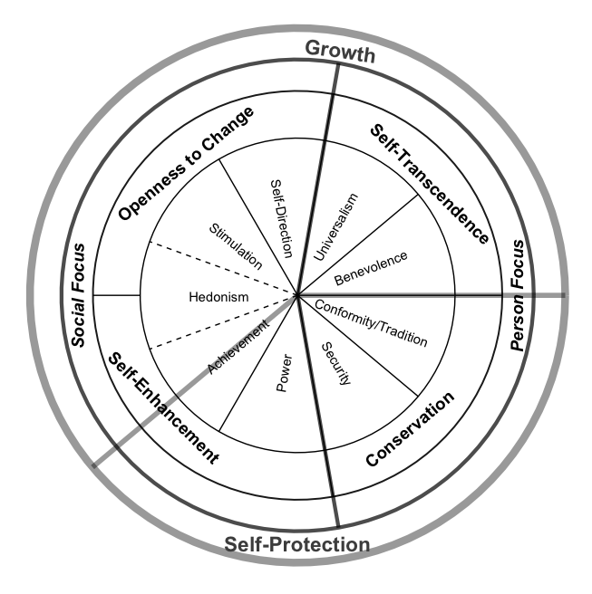
<ul>
  <li><code class="language-plaintext highlighter-rouge">add_circle()</code> - one argument is <code class="language-plaintext highlighter-rouge">r</code>, a radius. All the others are optional, passed to <code class="language-plaintext highlighter-rouge">geom_path</code>.</li>
  <li><code class="language-plaintext highlighter-rouge">add_radius()</code> - two arguments <code class="language-plaintext highlighter-rouge">angles.r1</code> is a vector of angles , <code class="language-plaintext highlighter-rouge">r1</code> is a length of line, <code class="language-plaintext highlighter-rouge">r0</code> is where the line begins, 0 by default. All the others are passed to <code class="language-plaintext highlighter-rouge">geom_segment</code>.</li>
  <li><code class="language-plaintext highlighter-rouge">add_label()</code>​ - <code class="language-plaintext highlighter-rouge">r</code> is radius, <code class="language-plaintext highlighter-rouge">angle.r</code> - vector of angles to which labels are located, <code class="language-plaintext highlighter-rouge">label</code> - vector of character labels, <code class="language-plaintext highlighter-rouge">pos</code> - position between center of circle and circle, by default is 1/2, which is middle. All others are optional and passed to <code class="language-plaintext highlighter-rouge">geom_text</code>; important is <code class="language-plaintext highlighter-rouge">angle</code> which accepts vectors and rotates the labels.</li>
</ul>

<pre><code class="language-{lang=&quot;rsplus&quot;}"># Value labels (easy to translate or abbreviate)
v9 &lt;- c("Security",
        "Conformity/Tradition",
        "Benevolence",
        "Universalism",
        "Self-Direction",
        "Stimulation",
        "Hedonism",
        "Achievement",
        "Power" )
v4 &lt;- c("Self-Transcendence",
        "Openness to Change",
        "Self-Enhancement",
        "Conservation")
v2_1 &lt;- c("Person Focus", "Social Focus")
v2_2 &lt;- c("Growth", "Self-Protection")
# Plotting
## Initial circle with radius 1
ggplot(data.frame(x = cos(seq(0,2*pi,length.out=100)),
                  y = sin(seq(0,2*pi,length.out=100))), aes(x,y))+coord_equal()+
  geom_path( col="black", linetype="solid")+
## Split circle into 8 sectors
  add_radius(seq(0, 360, 360/9)[c(1:4,7:9)], 1)+
## Label these 8 sectors
  add_label(r=1, angle.r=seq(1+20, 360-20, 319/8)[c(8,9,1:7)],
            label=v9,
            angle=seq(1+20, 360-20, 319/8)[c(8,9,1:7)]  %&gt;% sapply( function(x) if(x &gt; 90 &amp; x &lt; 270) x+180 else x  )      )+
## Hedonism dashed radiuses
  add_radius(seq(0, 360, 360/9)[5:6], r1=1, linetype="dashed")+
## Add another circle for higher order values OP-CO-SE-ST
  add_circle(r=1.3, linetype="solid", size=0.7, alpha=0.9)+
  add_radius(seq(0, 360, 360/9)[c(1,3, 8)], r0=1, r1=1.3)+add_radius(180, r0=1, r1=1.3, linetype="solid")+
  add_label(r=1.3, angle.r=seq(0+40, 360, 360/4),
            v4,
            angle=c(-45, 40, -45, 40),
            pos=0.85, fontface="bold", size = 5)+
## Yet another circles
  # Social-Person Focus
  add_circle(r=1.5, linetype="solid", size=1.5, alpha=0.7)+
  add_radius(seq(0, 360, 360/9)[c(3, 8)], r0=0, r1=1.5, size=1.5, alpha=0.7)+
  add_label(r=1.5, angle.r=c(0, 180), v2_1, angle=c(90, 90), pos=0.93, fontface="bold.italic", size = 5)+
  # Growth-Protection
  add_circle(r=1.7, linetype="solid", size=3, alpha=0.4)+
  add_radius(c(0, 220), r0=0, r1=1.7, size=2, alpha=0.4)+
  add_label(r=1.7, angle.r=c(90-10, 270), v2_2, angle=c(-8,0),
            pos=0.93, fontface="bold", size = 6, color="grey30")+
  theme_void()
</code></pre>

<p><img class="alignnone size-full wp-image-1589" src="/assets/images/uploads/2018/03/circle.png" alt="circle" width="653" height="656" /></p>]]></content><author><name></name></author><category term="blog" /><category term="r" /><summary type="html"><![CDATA[Since 2008 I draw Schwartz value theory in a form of circle unaccountable number of times, and there were very different versions, with more or fewer circles inside, in different languages and with different emphases. I used PowerPoint, Word, Excel, Paint, even Photoshop once. Here is not the optimal but quite universal and customizable solution. UPD. Now it’s a function schwartz_circle() in my R package LittleHelpers.]]></summary></entry><entry><title type="html">Branching pipes</title><link href="https://maksimrudnev.github.io/2018/03/04/branching-pipes-r/" rel="alternate" type="text/html" title="Branching pipes" /><published>2018-03-04T20:33:27+00:00</published><updated>2018-03-04T20:33:27+00:00</updated><id>https://maksimrudnev.github.io/2018/03/04/branching-pipes-r</id><content type="html" xml:base="https://maksimrudnev.github.io/2018/03/04/branching-pipes-r/"><![CDATA[<p>Here are three little functions that allow for brunching logical pipes as defined in <code class="language-plaintext highlighter-rouge">magrittr</code> package. It is against <a href="#hadley">Hadley’s idea</a>, as pipes are in principle linear, and in general I agree, but sometimes it would be comfy to ramify pipes away. It overcomes native <code class="language-plaintext highlighter-rouge">magrittr</code> <code class="language-plaintext highlighter-rouge">%T&gt;%</code> by allowing more than one step after cutting the pipe. Imagine you need to create a list with means, correlations, and regression results. And you like to do it in one single pipe. In general, it is not possible, and you’ll have to start a second pipe, probably doing some redundant computations. Here is an example that allows it:</p>

<pre><code class="language-{lang=&quot;rsplus&quot;}">data.frame(a=1:5, b=1/(1+exp(6:10)) ) %&gt;%
  ramify(1) %&gt;%
    branch(1) %&gt;% colMeans %&gt;%
    branch(2) %&gt;% lm(a ~ b, .) %&gt;% broom::tidy(.) %&gt;%
    branch(3) %&gt;% cor %&gt;%
      ramify(2) %&gt;%
        branch(1) %&gt;% round(2) %&gt;%
        branch(2) %&gt;% psych::fisherz(.) %&gt;%
      harvest(2) %&gt;%
  harvest
</code></pre>

<ul>
  <li><code class="language-plaintext highlighter-rouge">ramify()</code> - Saves current result into temporary object <code class="language-plaintext highlighter-rouge">.buf</code> and identifies a point in the pipe where branching will happen. Argument is an id of ramification.</li>
  <li><code class="language-plaintext highlighter-rouge">branch()</code> - Starts a new brunch from the <code class="language-plaintext highlighter-rouge">ramify</code> point. (brunch(1) can be omitted, as ramify creates the first brunch. Second argument is a family of branches, or parent branch. By default it uses the last parent branch created by last used <code class="language-plaintext highlighter-rouge">ramify</code>​.</li>
  <li><code class="language-plaintext highlighter-rouge">harvest()</code> - Returns contents of all the brunches as a list and clears the buffer.</li>
</ul>

<p><img class="alignnone size-full wp-image-1577" src="/assets/images/uploads/2018/03/branch.png" alt="BRANCH" width="1472" height="1442" /></p>

<p>See proof of concept <a href="https://gist.github.com/MaksimRudnev/bf81eab9f39bd830f9f167c669444472">https://gist.github.com/MaksimRudnev/bf81eab9f39bd830f9f167c669444472</a></p>

<hr />

<blockquote>
  <p><em>“Pipes are fundamentally linear and expressing complex relationships with them will typically yield confusing code.”</em> <em> <a href="http://r4ds.had.co.nz/pipes.html#when-not-to-use-the-pipe">http://r4ds.had.co.nz/pipes.html#when-not-to-use-the-pipe</a></em></p>
</blockquote>]]></content><author><name></name></author><category term="blog" /><category term="r" /><category term="LittleHelpers" /><summary type="html"><![CDATA[Here are three little functions that allow for brunching logical pipes as defined in magrittr package. It is against Hadley’s idea, as pipes are in principle linear, and in general I agree, but sometimes it would be comfy to ramify pipes away. It overcomes native magrittr %T&gt;% by allowing more than one step after cutting the pipe. Imagine you need to create a list with means, correlations, and regression results. And you like to do it in one single pipe. In general, it is not possible, and you’ll have to start a second pipe, probably doing some redundant computations. Here is an example that allows it: data.frame(a=1:5, b=1/(1+exp(6:10)) ) %&gt;% ramify(1) %&gt;% branch(1) %&gt;% colMeans %&gt;% branch(2) %&gt;% lm(a ~ b, .) %&gt;% broom::tidy(.) %&gt;% branch(3) %&gt;% cor %&gt;% ramify(2) %&gt;% branch(1) %&gt;% round(2) %&gt;% branch(2) %&gt;% psych::fisherz(.) %&gt;% harvest(2) %&gt;% harvest ramify() - Saves current result into temporary object .buf and identifies a point in the pipe where branching will happen. Argument is an id of ramification. branch() - Starts a new brunch from the ramify point. (brunch(1) can be omitted, as ramify creates the first brunch. Second argument is a family of branches, or parent branch. By default it uses the last parent branch created by last used ramify​. harvest() - Returns contents of all the brunches as a list and clears the buffer. See proof of concept https://gist.github.com/MaksimRudnev/bf81eab9f39bd830f9f167c669444472 “Pipes are fundamentally linear and expressing complex relationships with them will typically yield confusing code.”  http://r4ds.had.co.nz/pipes.html#when-not-to-use-the-pipe]]></summary></entry><entry><title type="html">‘n’go</title><link href="https://maksimrudnev.github.io/2018/02/16/ngo/" rel="alternate" type="text/html" title="‘n’go" /><published>2018-02-16T23:09:30+00:00</published><updated>2018-02-16T23:09:30+00:00</updated><id>https://maksimrudnev.github.io/2018/02/16/ngo</id><content type="html" xml:base="https://maksimrudnev.github.io/2018/02/16/ngo/"><![CDATA[<p><code class="language-plaintext highlighter-rouge">savengo</code> is ridiculously simple but potentially useful function that saves objects from a middle of your pipe and passes the same object to further elements of the pipe. It allows more efficient debugging and less confusing code, in which you don’t have to interrupt your pipe every time you need to save an output. Its sister function <code class="language-plaintext highlighter-rouge">appendngo</code> appends an intermediary product to an existing list or a vector. By analogy, one can create whatever storing function they need.</p>

<div class="language-plaintext highlighter-rouge"><div class="highlight"><pre class="highlight"><code># Example 1
#Saves intermediary result to an object named intermediate.result
final.result &lt;- dt %&gt;% dplyr::filter(score&lt;.5) %&gt;%
                        savengo("intermediate.result") %&gt;%
                        dplyr::filter(estimated&lt;0)
# Example 2
#Saves intermediary result as a first element of existing list
final.result &lt;- dt %&gt;% dplyr::filter(score&lt;.5) %&gt;%
                        appendngo(myExistingList, after=0) %&gt;%
                        dplyr::filter(estimated&lt;0)
</code></pre></div></div>

<p>See proof of concept <a href="https://gist.github.com/MaksimRudnev/bf81eab9f39bd830f9f167c669444472">https://gist.github.com/MaksimRudnev/bf81eab9f39bd830f9f167c669444472</a></p>]]></content><author><name></name></author><category term="blog" /><category term="r" /><summary type="html"><![CDATA[savengo is ridiculously simple but potentially useful function that saves objects from a middle of your pipe and passes the same object to further elements of the pipe. It allows more efficient debugging and less confusing code, in which you don’t have to interrupt your pipe every time you need to save an output. Its sister function appendngo appends an intermediary product to an existing list or a vector. By analogy, one can create whatever storing function they need. # Example 1 #Saves intermediary result to an object named intermediate.result final.result &lt;- dt %&gt;% dplyr::filter(score&lt;.5) %&gt;% savengo("intermediate.result") %&gt;% dplyr::filter(estimated&lt;0) # Example 2 #Saves intermediary result as a first element of existing list final.result &lt;- dt %&gt;% dplyr::filter(score&lt;.5) %&gt;% appendngo(myExistingList, after=0) %&gt;% dplyr::filter(estimated&lt;0) See proof of concept https://gist.github.com/MaksimRudnev/bf81eab9f39bd830f9f167c669444472]]></summary></entry><entry><title type="html">Little function to download ESS data on the go</title><link href="https://maksimrudnev.github.io/2017/12/15/little-function-to-download-ess-data-on-the-go/" rel="alternate" type="text/html" title="Little function to download ESS data on the go" /><published>2017-12-15T22:38:59+00:00</published><updated>2017-12-15T22:38:59+00:00</updated><id>https://maksimrudnev.github.io/2017/12/15/little-function-to-download-ess-data-on-the-go</id><content type="html" xml:base="https://maksimrudnev.github.io/2017/12/15/little-function-to-download-ess-data-on-the-go/"><![CDATA[<h3 id="motivation">Motivation</h3>

<p>Yes, there is a recently published brand new R package <a href="https://cran.r-project.org/web/packages/ess/vignettes/ess_r_stata_users.html"><code class="language-plaintext highlighter-rouge">ess</code></a> for downloading <a href="http://www.europeansocialsurvey.org/">European social survey data</a>, I tried it, although at this point it is quite limited. What are the good sides of <code class="language-plaintext highlighter-rouge">ess</code> package?</p>

<ul>
  <li>it downloads data, sometimes several data at a time</li>
</ul>

<p>What’s not so good?</p>

<ul>
  <li>when it downloads several rounds, you get a list of data instead of integrated dataset;</li>
  <li>it can only download one country data at a time;</li>
  <li>it tuned up for use in Stata, but not in R, for example, I couldn’t see most of the value labels.</li>
</ul>

<p>So, I thought it would be useful to have a customizable function (instead of package) to do the same thing, but better. For example, you can keep labels to use, for example, with my <a href="https://github.com/MaksimRudnev/LittleHelpers/tree/master/label_book">label_book</a>.</p>

<h3 id="details"><a id="user-content-details" class="anchor" href="https://gist.github.com/MaksimRudnev/5ffb5b412ea27e4af828d3f05ef68cf9#details"></a>Details</h3>

<p>Don’t put more than one country or more than one round - it won’t work. For countries, use <a href="https://en.wikipedia.org/wiki/ISO_3166-1_alpha-2">iso2c codes</a>, or “all”. This function will expire when ESS updates its data versions, but it happens about twice a year, and can be fixed manually.</p>

<h3 id="examples"><a id="user-content-examples" class="anchor" href="https://gist.github.com/MaksimRudnev/5ffb5b412ea27e4af828d3f05ef68cf9#examples"></a>Examples</h3>

<div class="language-plaintext highlighter-rouge"><div class="highlight"><pre class="highlight"><code>#1. Source the function
eval(parse(text =getURL("https://raw.githubusercontent.com/MaksimRudnev/LittleHelpers/master/download_ess/download_ess.R")))
#2. Enjoy it
ESS2 &lt;- download_ess(round=2, country="all", "mymail@gmail.com") #Add your registered on ESS website mail here
ESS6.Russia &lt;- download_ess(round=6, country="RU", "mymail@gmail.com")
</code></pre></div></div>

<h3 id="function-itself">Function itself</h3>

<!--more-->

<div class="language-plaintext highlighter-rouge"><div class="highlight"><pre class="highlight"><code>download_ess &lt;- function(round, country="all", user) {
 #1.Create url
 if(country!="all") {
 download.url &lt;- paste("http://www.europeansocialsurvey.org/file/download?f=ESS", round, country, ".spss.zip&amp;c=", country, "&amp;y=", round*2+2000, sep="")
 } else {
 version &lt;- c("06_5", "03_5", "03_6", "04_4", "03_3", "02_3", "02_1", "01")[round]
 download.url &lt;- paste("http://www.europeansocialsurvey.org/file/download?f=ESS", round, "e", version, ".spss.zip&amp;c=&amp;y=", round*2+2000, sep="")
 }
 #2. Download data
 library(httr)
 #Authenticate
 a&lt;-POST("http://www.europeansocialsurvey.org/user/login", body = list(u=user))
 # Download
 data.file &lt;- GET(download.url)
 # Write temporary file
 writeBin(content(data.file, "raw"), paste(tempdir(), "file.zip"))
 # Unzip
 path&lt;-utils::unzip(paste(tempdir(), "file.zip"))
 #3. Read in with haven package
 haven::read_spss(path[length(path)])
}
</code></pre></div></div>

<p>UPD. Now these functions are a part of my R package <em><a href="https://github.com/MaksimRudnev/LittleHelpers/">LittleHelpers</a>.</em></p>]]></content><author><name></name></author><category term="blog" /><category term="r" /><category term="European Social Survey" /><summary type="html"><![CDATA[Motivation Yes, there is a recently published brand new R package ess for downloading European social survey data, I tried it, although at this point it is quite limited. What are the good sides of ess package? it downloads data, sometimes several data at a time What’s not so good? when it downloads several rounds, you get a list of data instead of integrated dataset; it can only download one country data at a time; it tuned up for use in Stata, but not in R, for example, I couldn’t see most of the value labels. So, I thought it would be useful to have a customizable function (instead of package) to do the same thing, but better. For example, you can keep labels to use, for example, with my label_book. Details Don’t put more than one country or more than one round - it won’t work. For countries, use iso2c codes, or “all”. This function will expire when ESS updates its data versions, but it happens about twice a year, and can be fixed manually. Examples #1. Source the function eval(parse(text =getURL("https://raw.githubusercontent.com/MaksimRudnev/LittleHelpers/master/download_ess/download_ess.R"))) #2. Enjoy it ESS2 &lt;- download_ess(round=2, country="all", "mymail@gmail.com") #Add your registered on ESS website mail here ESS6.Russia &lt;- download_ess(round=6, country="RU", "mymail@gmail.com") Function itself]]></summary></entry><entry><title type="html">Label book for R</title><link href="https://maksimrudnev.github.io/2017/11/01/label-book-for-r/" rel="alternate" type="text/html" title="Label book for R" /><published>2017-11-01T14:59:41+00:00</published><updated>2017-11-01T14:59:41+00:00</updated><id>https://maksimrudnev.github.io/2017/11/01/label-book-for-r</id><content type="html" xml:base="https://maksimrudnev.github.io/2017/11/01/label-book-for-r/"><![CDATA[<p>Sometimes, when you explore a new dataset, variable names don’t make much sense. In SPSS you would just look at the labels, in R it’s not that straightforward: checking codebooks all the time is tedious, reading a questionnaire and trying to guess which variable corresponds to each question is even less reliable. If your data has labels as attributes, or you have read .sav datafile into R with <code class="language-plaintext highlighter-rouge">haven</code> or <code class="language-plaintext highlighter-rouge">foreign</code> package, it would be handy to have a searchable table of all the variable and value labels in the dataset. I looked it up and didn’t find such a function, so I have written a little simple function myself.   <em><strong>UPD.</strong> Now this function is a part of my R package <a href="https://github.com/MaksimRudnev/LittleHelpers/">LittleHelpers</a>.</em> <!--more--> The function gets the attributes of variables and value labels and put them in a nicely formatted table.</p>

<p>##</p>

<p>Use: <code class="language-plaintext highlighter-rouge">label_book(df, max.val=25, vars="all", view=TRUE)</code> There are three arguments:</p>

<ul>
  <li><code class="language-plaintext highlighter-rouge">df</code> - data.frame, result of reading spss file by packages ‘haven’ or ‘foreign’</li>
  <li><code class="language-plaintext highlighter-rouge">max.vals</code> - integer, how many value labels per each variable shoud be listed in the table, default is 25</li>
  <li><code class="language-plaintext highlighter-rouge">vars</code> - can be integer, character, or range of integers or characters. Variables indexes or names for getting subsets of label book.</li>
  <li><code class="language-plaintext highlighter-rouge">view</code> - logical, whether the result should be shown in the RStudio viewer pane. Defualt is TRUE. If FALSE, html file named <em>‘label_book_output.html’</em> is saved in your working directory.</li>
</ul>

<p>The only extra package required is <code class="language-plaintext highlighter-rouge">knitr</code>.</p>

<h2 id="example"><a id="user-content-example" class="anchor" href="https://github.com/MaksimRudnev/LittleHelpers/blob/master/label_book/readme.md#example"></a>Example</h2>

<div class="highlight highlight-source-r">

    # Read the data
     ess8&lt;- haven::read_sav("ESS8e01.sav")
    # Download the function
     eval(parse(text=getURL("https://raw.githubusercontent.com/MaksimRudnev/LittleHelpers/master/label_book/label_book.R")))
    # Use the function
     label_book(ess8, max.vals=11, vars=45:50)

</div>

<h2 id="result"><a id="user-content-result" class="anchor" href="https://github.com/MaksimRudnev/LittleHelpers/blob/master/label_book/readme.md#result"></a>Result</h2>

<h1 id="label-book-for-ess8"><a id="user-content-label-book-for-ess8" class="anchor" href="https://github.com/MaksimRudnev/LittleHelpers/blob/master/label_book/readme.md#label-book-for-ess8"></a>Label Book for “ess8”</h1>

<table> <thead> <tr> <th>Variables</th> <th>Variable labels</th> <th>Values</th> <th>Value labels</th> </tr> </thead> <tbody> <tr> <td>contplt</td> <td>Contacted politician or government official last 12 months</td> <td>1</td> <td>Yes</td> </tr> <tr> <td></td> <td></td> <td>2</td> <td>No</td> </tr> <tr> <td></td> <td></td> <td>7</td> <td>Refusal</td> </tr> <tr> <td></td> <td></td> <td>8</td> <td>Don't know</td> </tr> <tr> <td></td> <td></td> <td>9</td> <td>No answer</td> </tr> <tr> <td>wrkprty</td> <td>Worked in political party or action group last 12 months</td> <td>1</td> <td>Yes</td> </tr> <tr> <td></td> <td></td> <td>2</td> <td>No</td> </tr> <tr> <td></td> <td></td> <td>7</td> <td>Refusal</td> </tr> <tr> <td></td> <td></td> <td>8</td> <td>Don't know</td> </tr> <tr> <td></td> <td></td> <td>9</td> <td>No answer</td> </tr> <tr> <td>wrkorg</td> <td>Worked in another organisation or association last 12 months</td> <td>1</td> <td>Yes</td> </tr> <tr> <td></td> <td></td> <td>2</td> <td>No</td> </tr> <tr> <td></td> <td></td> <td>7</td> <td>Refusal</td> </tr> <tr> <td></td> <td></td> <td>8</td> <td>Don't know</td> </tr> <tr> <td></td> <td></td> <td>9</td> <td>No answer</td> </tr> <tr> <td>badge</td> <td>Worn or displayed campaign badge/sticker last 12 months</td> <td>1</td> <td>Yes</td> </tr> <tr> <td></td> <td></td> <td>2</td> <td>No</td> </tr> <tr> <td></td> <td></td> <td>7</td> <td>Refusal</td> </tr> <tr> <td></td> <td></td> <td>8</td> <td>Don't know</td> </tr> <tr> <td></td> <td></td> <td>9</td> <td>No answer</td> </tr> <tr> <td>sgnptit</td> <td>Signed petition last 12 months</td> <td>1</td> <td>Yes</td> </tr> <tr> <td></td> <td></td> <td>2</td> <td>No</td> </tr> <tr> <td></td> <td></td> <td>7</td> <td>Refusal</td> </tr> <tr> <td></td> <td></td> <td>8</td> <td>Don't know</td> </tr> <tr> <td></td> <td></td> <td>9</td> <td>No answer</td> </tr> <tr> <td>pbldmn</td> <td>Taken part in lawful public demonstration last 12 months</td> <td>1</td> <td>Yes</td> </tr> <tr> <td></td> <td></td> <td>2</td> <td>No</td> </tr> <tr> <td></td> <td></td> <td>7</td> <td>Refusal</td> </tr> <tr> <td></td> <td></td> <td>8</td> <td>Don't know</td> </tr> <tr> <td></td> <td></td> <td>9</td> <td>No answer</td> </tr> </tbody> </table>]]></content><author><name></name></author><category term="blog" /><category term="r" /><summary type="html"><![CDATA[Sometimes, when you explore a new dataset, variable names don’t make much sense. In SPSS you would just look at the labels, in R it’s not that straightforward: checking codebooks all the time is tedious, reading a questionnaire and trying to guess which variable corresponds to each question is even less reliable. If your data has labels as attributes, or you have read .sav datafile into R with haven or foreign package, it would be handy to have a searchable table of all the variable and value labels in the dataset. I looked it up and didn’t find such a function, so I have written a little simple function myself.   UPD. Now this function is a part of my R package LittleHelpers.]]></summary></entry></feed>